Deng et al.(2021): Social network analysis of virtual water trade among major countries in the world

💡 1. Research Question and Research Gap

What is the structure of the virtual water trade network between major countries in the world?

Previous studies have primarily focused on virtual water trade related to agricultural products. Also, most of them have simply compared the total import and export volumes by country. This study introduces a methodology called Social Network Analysis to quantitatively analyze the structural characteristics of virtual water trade and provides an integrated analysis of virtual water trade networks across the entire industrial structure.

🌊 2. Introduction

Why is virtual water trade important?

Water is a key resource that supports all industries, agriculture, and daily life. However, the problem is that water is very disproportionately distributed among countries. That’s where the concept of Virtual Water Trade comes in. It refers to the idea that when we trade goods, we are also indirectly trading the water used to produce them. This study shows how virtual water trade plays a role in solving water shortages between countries and explores how the global trade network is connected in terms of virtual water flows.

🔧 3. Methods and Data Sources

💡 How is Virtual Water calculated?

This study estimates inter-country virtual water flows using a Multi-Regional Input–Output (MRIO) model.

Direct Water Coefficient

\[ w_i^r = \frac{W_i^r}{X_i^r} \]

• \(W_i^r\): Water consumed by industry i in country r
• \(X_i^r\): Total output of industry i in country r
  -> how much water is used to produce one unit of output

Input–Output Balance Equation

\[ AX + Y = X \]

• \(A\): Input coefficient matrix (inter-industry consumption)
• \(X\): Total output vector
• \(Y\): Final demand vector
  -> Total output equals intermediate + final consumption

Leontief Inverse Matrix

\[ X = (I - A)^{-1}Y = LY \]

• \(L = (I - A)^{-1}\): Leontief inverse matrix
  -> Both direct and indirect production requirements

Virtual Water Trade Matrix

\[ H = \hat{W} \cdot L \cdot Z \]

• \(\hat{W}\): Diagonal matrix of direct water coefficients
• \(L\): Leontief inverse
• \(Z\): Final goods traded between countries
  -> estimate indirect virtual water flows across borders

Virtual Water Network Matrix

\[ T = H \]

• \(t_{rs}\): Virtual water exported from country r to country s
  -> Off-diagonal elements show bilateral virtual water trade

📊 4. Network Analysis: How Virtual Water Trade is Structured

To analyze the structure of the virtual water trade, this study applies social network metrics:

Density (Network Connectivity)

\[ D = \frac{\sum_{r \neq s} \sum_{s=1}^{m} t_{rs}}{m(m - 1)} \]

• Measures how densely connected the virtual water network is
• Higher values = more active trade across countries

Asymmetry (Trade Imbalance)

\[ S = \frac{\sum_{r \neq s} \sum_{s=1}^{m} |t_{rs} - t_{sr}|}{m(m - 1)} \]

• Capture the imbalance between exports and imports
• High values = unidirectional or one-sided trade

Out-Degree (Virtual Water Exports)

\[ OD_r = \sum_{s \neq r} t_{rs} \]

• Total virtual water exported by country r
• Indicates water-exporting hubs

In-Degree (Virtual Water Imports)

\[ ID_r = \sum_{s \neq r} t_{sr} \]

• Total virtual water imported into country r
• High values suggest greater water dependency

🎯 5. Result and Interpretation

Global virtual water trade has continuously increased from 2006 to 2015. Both virtual water exports and imports increased significantly from 2006 to 2015, showing a clear growth in global trade among major countries.

<Network by Out-Degree (2015)>

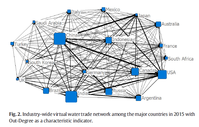
The Out-Degree network shows countries that exported large amounts of virtual water to others. China and India had the largest outflows, shown by the largest node sizes and thick outbound links. This indicates that these countries acted as central suppliers in the global virtual water trade network.

<Network by In-Degree (2015)>

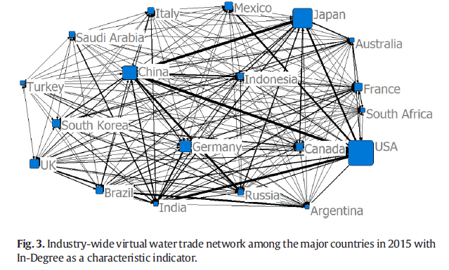
The In-Degree network focuses on countries with high virtual water imports. The United States and Japan had the biggest consumers, shown by the largest node sizes and thick incoming links. These countries had strong dependencies on foreign water resources embedded in traded goods.

📍 6. Conclusions

Virtual water trade can be an important way to reduce water resource differences between countries around the world Using Social Network Analysis, this study identifies key structural features of virtual water flows and highlights central players in the trade network. As a result of the analysis, China is a major exporter and the United States is a major importer, serving as a key hub for the virtual water network. In particular, virtual water trade was the most active in the agricultural sector, suggesting that trade strategies in the agricultural sector are important in policy.

A Network Analysis of Global Wine🍷 and Beer🍺 Trade

📦 Data Introduction

Data Sources

The dataset was obtained from the FAOSTAT platform. FAOSTAT is an official platform of the Food and Agriculture Organization (FAO) that provides free access to global food and agriculture statistics. It covers over 245 countries and territories and includes long-term data starting from 1961. For this project, I used trade data to analyze virtual water flows related to wine and beer. Node-level information was constructed using population, GDP per capita, and foreign direct investment (FDI) datasets.

Major Characteristics of the Data

1. Time Range (1990–2023)
   • The dataset covers global trade from 1990 to 2023.
   • This allows for a long-term analysis of how virtual water flows have changed over time, especially in the trade of wine and beer.

1. Focus on Selected Items
   • Two beverage-related items were selected from FAOSTAT trade data:
     • Wine
     • Beer of barley, malted

1. Edge Data
   • Based on FAOSTAT’s detailed bilateral trade matrix.
   • Each trade record includes reporter/partner country, reporter/partner code, year, item, unit, and trade value.
   • Trade flows were filtered with the following conditions:
     • Year: 1990–2023
     • Final Value > 1000 (to retain only meaningful trade relationships)

1. Node Data

   • The following three datasets were merged to construct the node attributes:

     • Population_E_All_Data_(Normalized).csv
       -> Selected element: Total Population - Both sexes

     • Macro-Statistics_Key_Indicators_E_All_Data_(Normalized).csv
       -> Selected element: Value US$ per capita (GDP per Capita)

     • Investment_ForeignDirectInvestment_E_All_Data_(Normalized).csv
       -> Selected item: Total FDI inflows, element: Value US$

   • These attributes add demographic, economic, and investment information to each country node.

Data Pre-processing

1. Link
Filter by Export/Import and Items
Focus only on two beverage products: Wine and Beer made from barley, malted.
Filter the dataset to include only export and import records with positive values.

# Export data
link2 = link[(link['Element'] == 'Export quantity') & (link['weight'] > 0)]
items_export = link2[(link2['item'] == 'Wine') | (link2['item'] == 'Beer of barley, malted')]

# Import data
link3 = link[(link['Element'] == 'Import quantity') & (link['weight'] > 0)]
items_import = link3[(link3['item'] == 'Wine') | (link3['item'] == 'Beer of barley, malted')]

Merge Export & Import
Merge export and import datasets on matching country pairs, items, and years.
Calculate the Final Value by choosing the larger of export and import values for each trade pair.

link_merge = pd.merge(items_export, items_import,
    on=["O_code", "O_name", "D_code", "D_name", "item", "year"],
    how='inner')

link_merge["Final Value"] = np.where(link_merge["weight_x"] > link_merge["weight_y"],
                                     link_merge["weight_x"], link_merge["weight_y"])

2. Node
Merge the three datasets

# Merge Population and GDP
node_df = pop1.merge(macro1, on=["country", "country_code", "Year"], how="inner")

# Merge with FDI data
node_df = node_df.merge(fdi1, on=["country", "country_code", "Year"], how="inner")

# Choose final columns
node_df = node_df[["country", "country_code", "Year", "population", "GDP", "FDI"]]
node_df

📈 Analysis

Density Plot

Wine (red line): The network density of wine has been steadily increasing since the early 1990s. It shows a continuous trend of increasing overall. In particular, it has shown a sharp increase since 2020, indicating that wine is emerging as a major central item in the virtual water resource trade. This means that wine-producing countries are actively trading with various countries, forming tighter trade networks.
Beer (blue line): Beer has seen a rather modest increase since the mid-1990s, maintaining a lower network density than wine. Although it has increased somewhat since 2020, it is still lower than wine. This means that it is an item with relatively less trade connectivity.
Overall interpretation: The marked increase in network density since 2020 for both wine and beer reflects the impact of boosting global trade and improving logistics infrastructure. Wine maintains trade relations with more countries, suggesting it is positioned as a central item in the virtual water flow.

Wine

2023 In Degree / Out Degree

As of 2023, Germany, the United Kingdom, and the United States accounted for the largest share of the global wine import market. These countries have a steady demand for imports based on their long wine consumption culture and stable purchasing power. The Netherlands and Belgium are also among the top countries, showing that wine consumption is very active in Europe.

In the 2023 wine export market, Italy, Spain, and France accounted for the majority of global wine exports as traditional wine powerhouses. With major European-focused producers still leading the global market, Australia is at the top of the list and growth in non-European countries can also be seen. In addition, Germany is among the top five countries not only in imports but also in exports, so both production and consumption are actively taking place.

Top 5 Countries by In Degree / Out Degree (1990–2023)

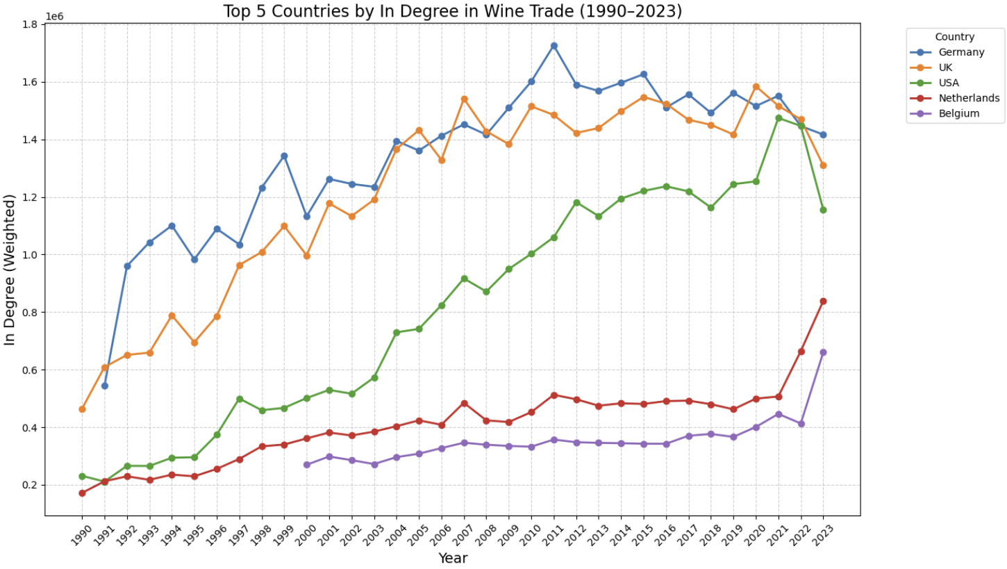
Since the 1990s, Germany and the United Kingdom have established themselves as major consumers of the global wine market with consistently high wine imports. The U.S. has emerged as the world’s third-largest importer, showing a steep increase since the mid-2000s. Belgium and the Netherlands have also maintained steady gains and hold important positions in Europe-focused wine import networks.

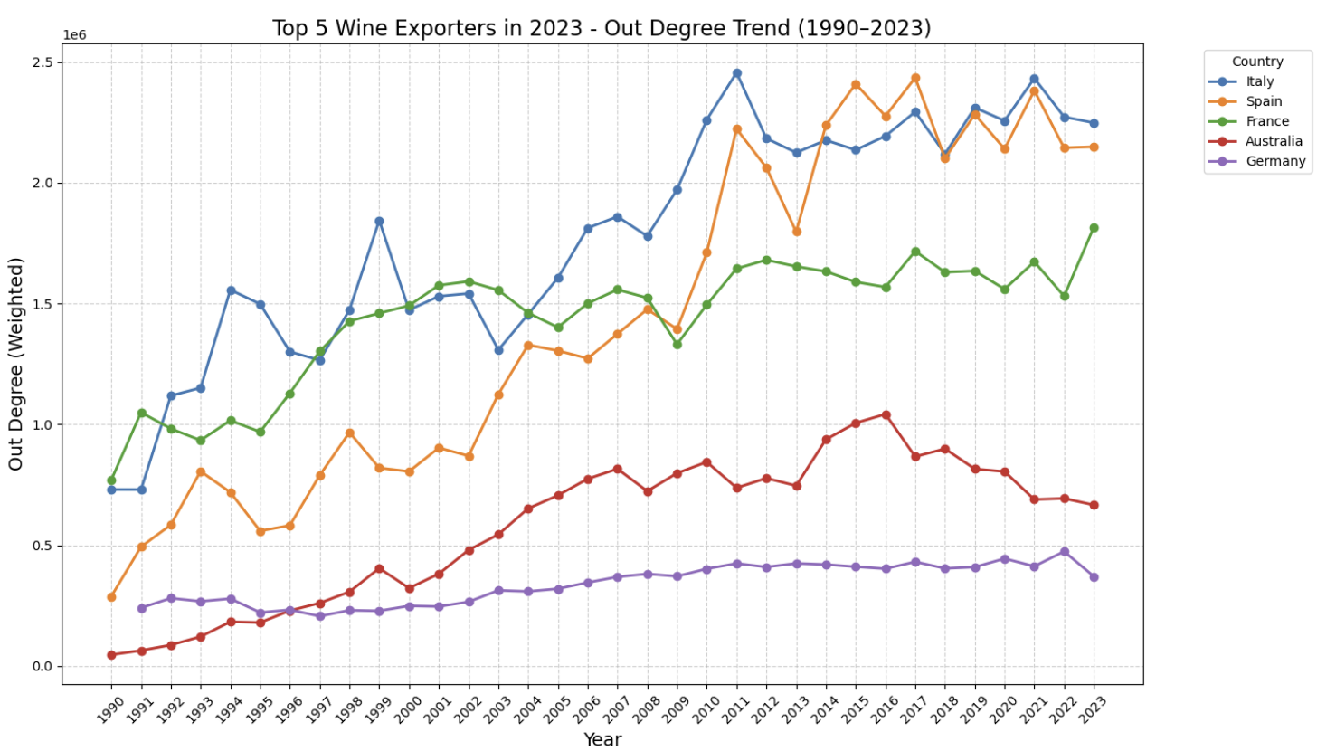
Italy and Spain have maintained their leadership positions for over 30 years, demonstrating their status as traditional wine export powers. France also maintains high export volumes as a traditional producer, with major European countries still leading the global supply chain. Australia has grown rapidly since the 2000s and has become a representative exporter of non-European countries. Germany remains at the top of the list in terms of exports, making it an active country for both production and consumption.

Beer

2023 In Degree / Out Degree

In the 2023 beer import market, the U.S. topped the list with overwhelming imports. France, the United Kingdom and Italy also saw high imports, meaning that the culture of beer consumption in Europe remains active. In particular, the Netherlands is at the top of the list of imports as well as beer exports, showing that it is playing a dual role.

Mexico has emerged as a hub of global beer supply, dominating the beer export market in 2023. Following this, the Netherlands, Belgium and Germany remain at the top, indicating that European countries are still leading global beer production and exports. Ireland is also among the top five countries, solidifying its position as a traditional beer producer.

Top 5 Countries by In Degree / Out Degree (1990–2023)

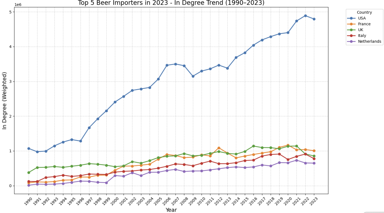
Since 1990, the U.S. has steadily increased its beer imports, making it an unrivaled No. 1 spot in 2023. France, Britain, Italy and the Netherlands remained at the top, showing stable import flows across the board, although there were slight fluctuations. Import trends in European countries, in particular, indicate that the culture of beer consumption in Europe continues to be maintained.

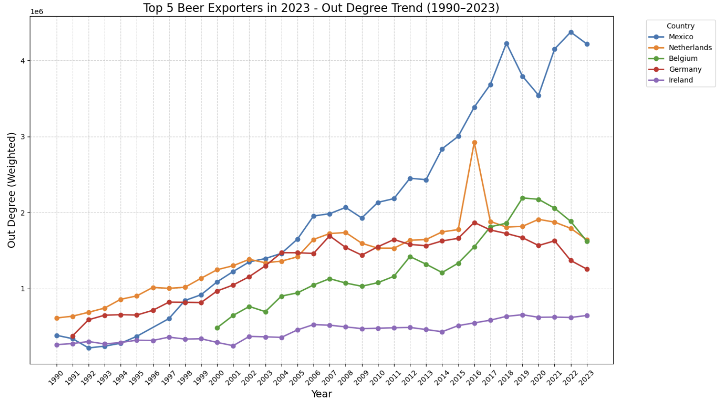
Mexico has rapidly expanded its exports since the early 2000s, emerging as a strong player in the global beer export market since 2010. As traditional beer producers, the Netherlands and Belgium maintained their position as major exporters, maintaining steady export volumes. Germany and Ireland also showed stable growth and were among the top five countries in 2023.

🧠 Network Visualization

To reduce complexity, only the top 30 countries (by connectivity) are shown in each network. Node size and color help highlight each country’s role and trading patterns in the global wine and beer trade. These visualizations allow us to better understand trade hubs, key intermediaries, and regional trading communities.

Wine Trade Network

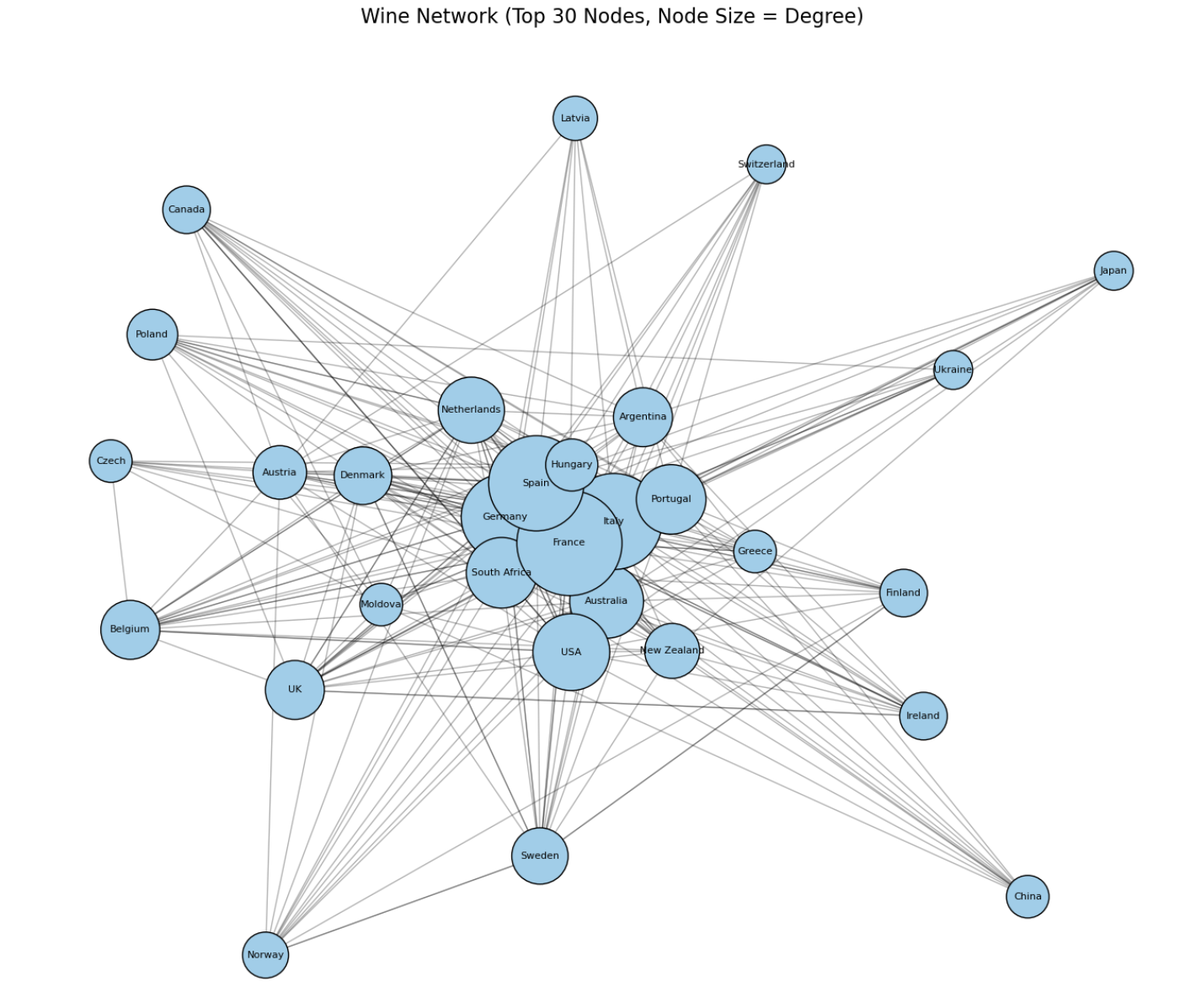
This graph represents the overall connection centrality, and the size of the node represents the total number of connections in that country. Major European countries such as France, Germany, Italy and Spain are located at the center of the network, showing active trade activity. The larger the nodes, the more countries we are trading wine with, and these countries act as hubs for our global wine network.

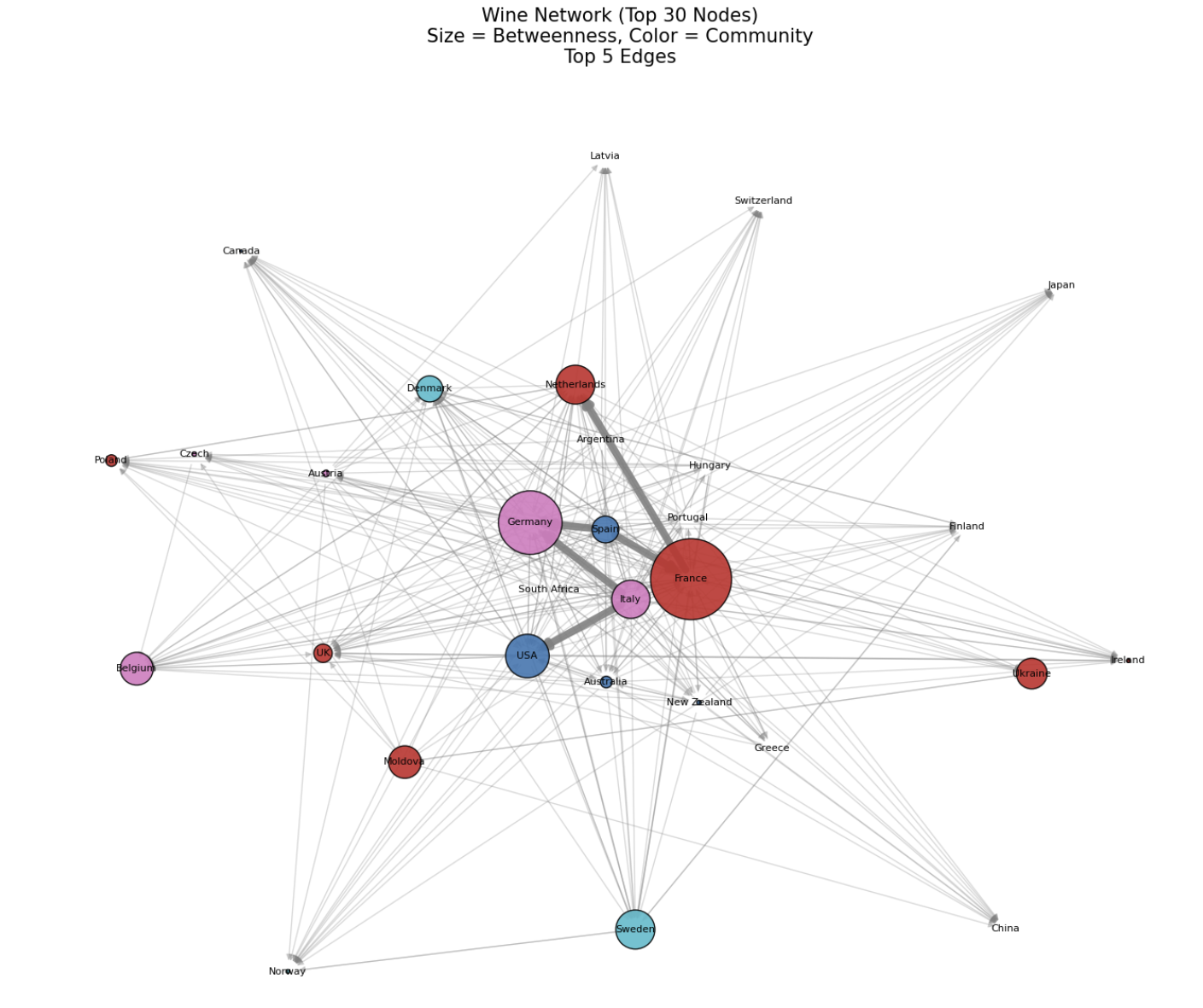
The size of a node is the betweenness centrality, which indicates how important intermediaries one country plays in trade routes between other countries. France and Germany appeared to be key transit stations connecting the main routes, showing that they hold strategic positions in the global wine trade. Colors represent community structures, and countries with similar trade patterns are tied together in the same color. This allows you to identify trade communities formed by regions such as Europe, Asia, and Oceania. The thickest lines represent the Top 5 Edges, highlighting the strongest trade connections between country pairs. These edges reveal high mutual dependency and help identify the most significant trade routes in the global wine network.

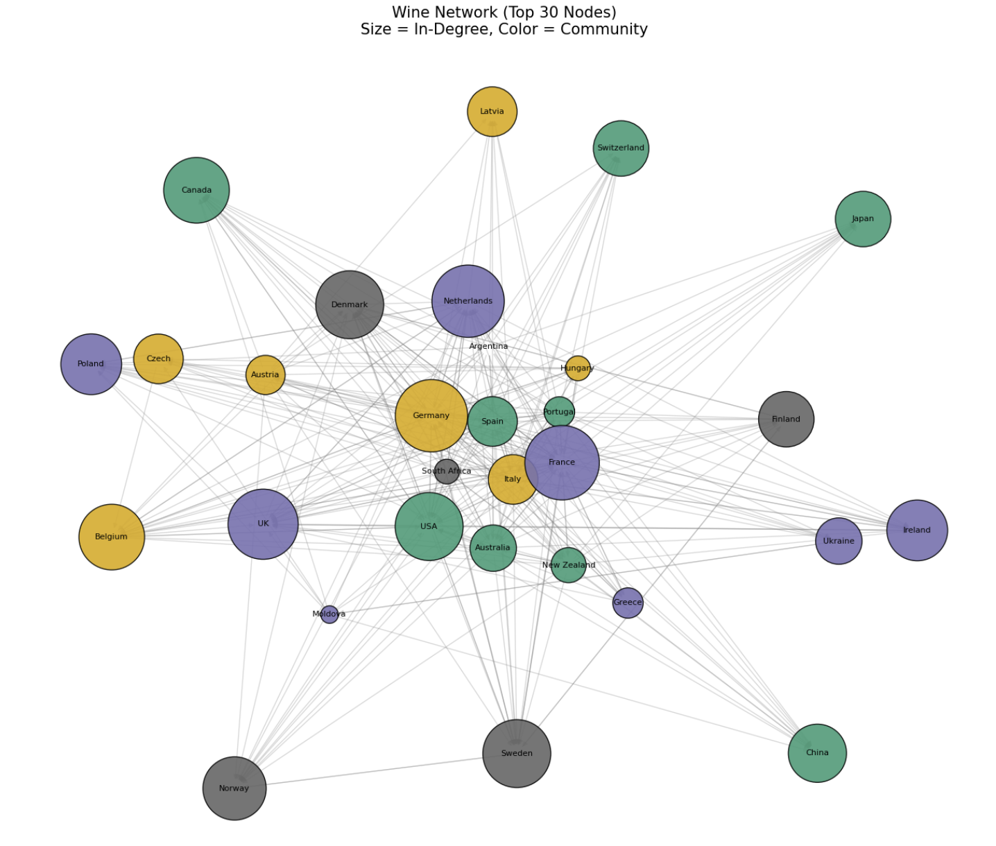
Node size represents In-Degree (number of import-oriented connections). Germany, France, Canada and the United Kingdom import wine from a number of countries and are at the heart of the import network. Community color analysis can identify which trade group the major importing countries belong to, and European countries tend to be mostly in the same community.

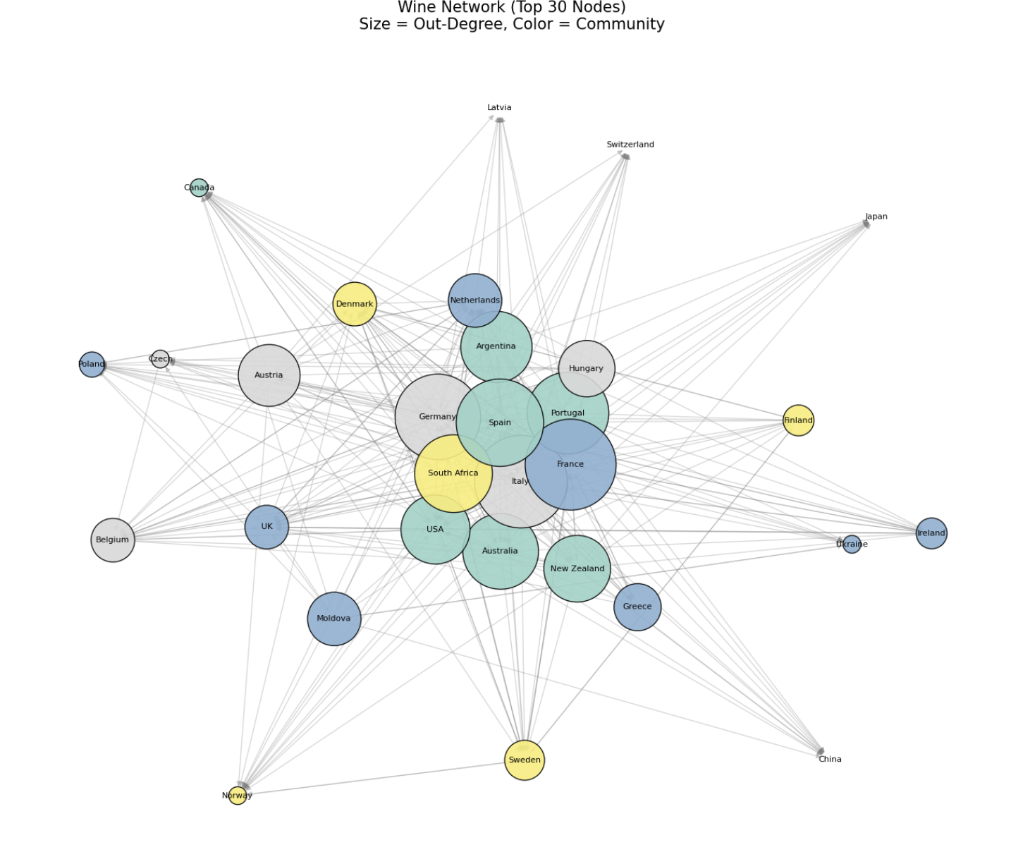
The size of the node means Out-Degree, and major producers such as France, Italy, and Spain appear as large nodes. These countries export wine to a variety of countries, and are key to the global supply side network. As a result of community analysis, trade connections between European countries are very close, and export-oriented countries share similar patterns with each other.

Beer Trade Network

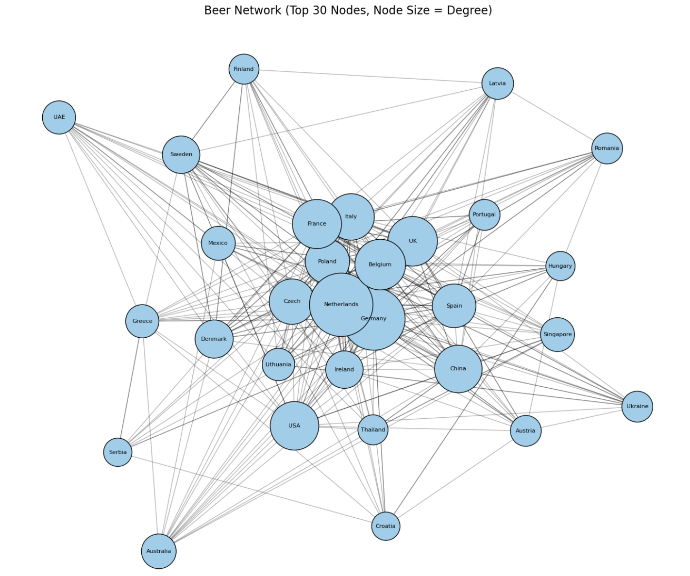
This graph is a network created based on the degree of connection (Degree) of each country. The larger the node, the more countries we have beer trade relationships with. Germany, the Netherlands, France and the United Kingdom are among the major hub countries with active beer trade, with locations centered on trade networks. It can be visually confirmed that they are playing a central role in the global beer trade.

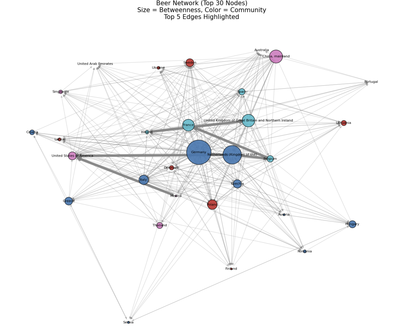
The size of the node is the betweenness centrality, which shows how important intermediaries one country plays in the trade routes between other countries. Germany and the U.K. appeared to be key transit stations connecting the main routes, suggesting they hold strategic positions in the global beer trade. Colors represent community structures, and countries that share similar trade patterns are grouped together in the same color. This allows you to understand the distribution of trade groups by region (e.g., Europe, Asia, etc.). In particular, the boldest lines represent the Top 5 Edges, which show the trade relationships between the most mutually dependent country pairs. This strong connection could be interpreted as the most important trade route within the global beer network.

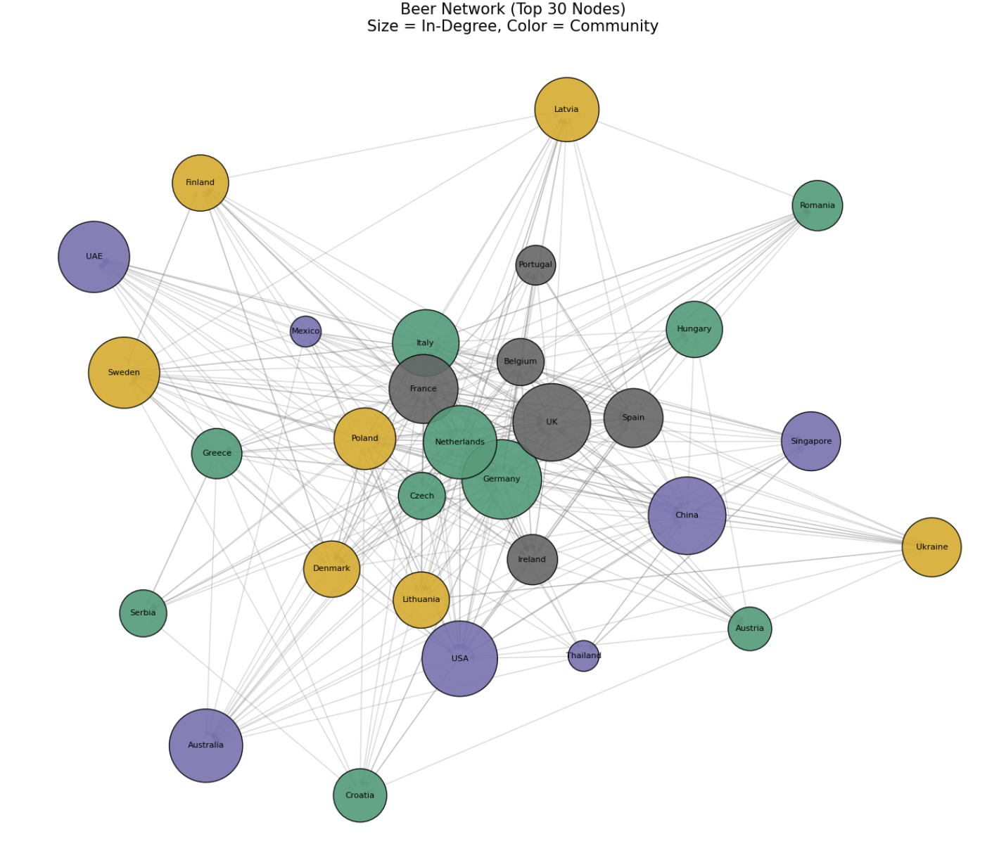
In this visualization, the size of the node represents In-Degree. In other words, it is an indicator of how many countries are importing beer from. The U.S., France, the U.K., and Italy were the major importers with high In-Degrees. Community color analysis also enables visual identification of trade groups to which major importers belong, and can infer regional consumption centers.

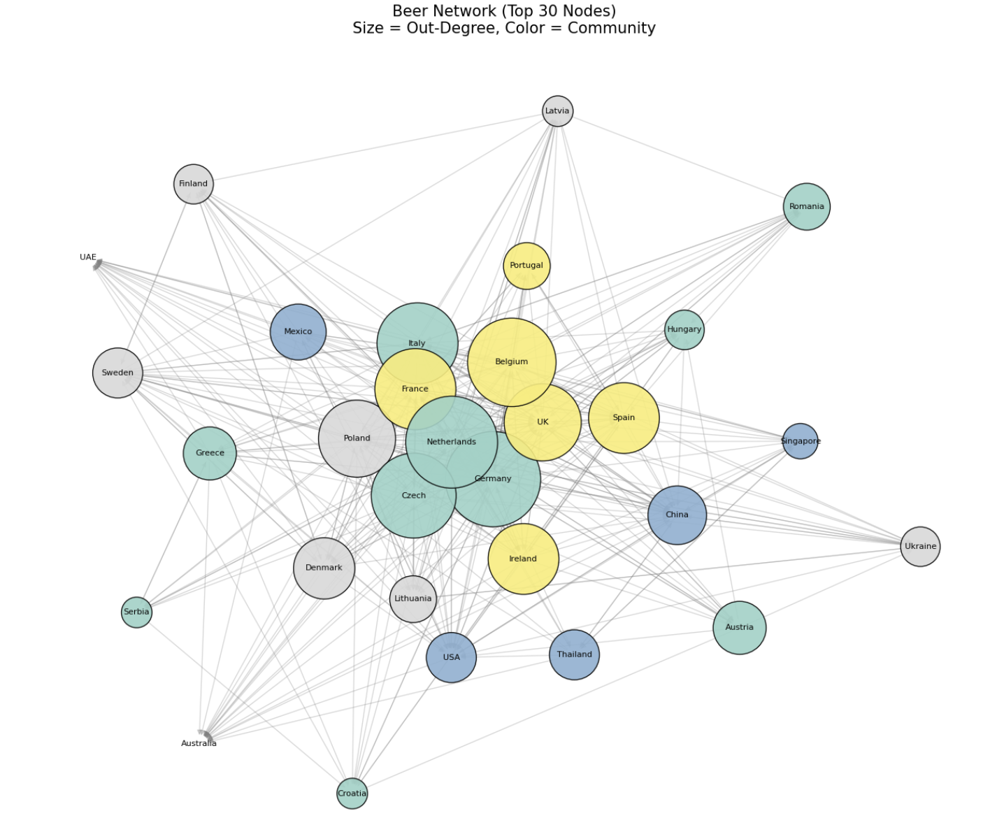
The size of the node represents the Out-Degree (number of export connections). Traditional beer export powers such as Germany, Belgium, the Netherlands, and France are represented by large nodes, and they are global supply-oriented countries in that they export beer to various countries. The colors represent the community affiliation of each country, suggesting that countries with similar export routes form one trading bloc. This allows us to understand the close trade relationship between export-focused countries in Europe.

Comparison of Wine and Beer Trade Networks

Both wine and beer networks have been visualized based on the top 30 countries, but they show distinct differences in structural characteristics, composition of central countries, and trade flows. The wine network is very densely connected around Europe, with traditional wine producers such as France, Italy, Germany, and Spain at the center of the network. They have a strong influence on exports, while Germany, the United Kingdom, and the United States are at the center of In-Degree as major importers. In the case of wine, the distinction between exporting and importing countries is relatively clear.

On the other hand, the beer network has a more decentralized structure and includes not only Europe, but also various regional countries such as the United States, Mexico, and China. Germany, the Netherlands, and the United Kingdom are strong exporters and at the same time record high imports, with active two-way trade. Germany, in particular, occupies a central position in both exports and imports, showing a greater emphasis on the role of intermediary than in the wine network.

In terms of centrality, in wine, France and Germany appear as major transit stations connecting trade routes between countries, with high betweenness centrality. Germany and the U.K. play similar roles in beer networks, but as a whole, various countries tend to be dispersed as intermediaries. The community structure is also different, with wine networks having more diverse communities while European countries form one dense community, and countries in Asia and the Americas also forming distinct groups.

As a result, we can see that wine trade has a strong traditional producer-oriented structure, while beer trade has formed a more open and multipolar global network. This reflects the difference in the production and consumption culture of the two commodities, as well as the logistics infrastructure, and provides important implications for understanding the multifaceted nature of global food trade.

🌍 Mapping

A map-based network was formed to visually understand the flow of the world’s wine and beer trade. It has reduced complexity and emphasized core trade flows by leaving only the strongest trade connections with the top 10 major country nodes. It is an intuitive visualization that provides a quick understanding of the centrality and interdependence of trade between countries. It provides much more intuitive insights than simple numerical data because it shows the direction and scale of the flow together on the map.

Global Wine Trade

The wine trade network centered around Europe is clearly visible. Traditional wine-producing countries such as France, Germany and Italy appear as central nodes, and export flows from these countries to various regions are concentrated. The routes between some of the countries, with the thickest trade lines, reflect a high trade dependence, and show a scalable trade structure from Europe to North America and Asia. In particular, trade between European internal countries is closely conducted, suggesting the possibility of intra-regional trade bloc formation.

Global Beer Trade

Beer trade appears in a more decentralized form than wine, showing an active trade flow between Europe, North America, and Asia and Oceania. Germany, the United States, and the Netherlands act as central hubs, while non-European countries such as Australia, Singapore, and Thailand also appear as major nodes. These structures visually demonstrate that the global beer industry is multipolar around various consumer markets and production bases. In particular, the strength of the connection between Europe and Asia is remarkable, and its strategic position in the global supply chain can be identified.

🧾 Summary and Key Insights

This project is an example of analyzing the virtual water trade structure centered on wine and beer through social network analysis (SNA) techniques. Based on FAOSTAT trade data from 1990 to 2023, item filtering, preprocessing, and node/link data were constructed, Since then, major network indicators such as connection strength, centrality, and community structure have been comprehensively analyzed. Network visualization and map-based analysis allowed us to see at a glance the role of key countries and the strategic location of trade flows. As a result, wine had a centralized network centered on traditional European producers, and beer had a multipolar structure involving various countries. In addition, centrality and community analysis have found that certain countries are acting as “hubs” or “intermediaries” in their networks beyond simple trade partners. In particular, map-based visualizations provide intuitive understanding of the flow of global trade, effectively revealing key trade routes and interdependencies.