Andris et al. (2023): Human-network regions as effective geographic units for disease mitigation

💡 1. Research Question and Research Gap

To what extent do human mobility-based regions serve as more effective geographic units for mitigating the spread of COVID-19 than administrative boundaries?

Administrative units (state boundaries) often fail to capture the actual scope of human activity. This study defines functional regions by applying community detection algorithms to networks of human movement and social connections (such as commutes, GPS-based trips, and social media ties), and compares how effectively these alternative boundaries mitigate the spread of infectious diseases.

🌊 2. Introduction

The COVID-19 pandemic has highlighted the impact of interregional movement on the spread of infectious diseases, which has raised the issue that it is difficult to design effective quarantine policies only with existing administrative boundaries. In particular, if the same living area spans multiple administrative districts, different quarantine guidelines may conflict and lead to inefficiency. As an alternative to overcome these limitations, this study proposes functional areas based on human movement as a new policy unit.

🌐 3. Data and Methodology

📦 Human-Network Datasets

Five networks were constructed at the county level in the contiguous U.S.:

• Commutes
• Trips
• Migration
• Twitter
• Facebook

Nodes represent U.S. counties.
Edges represent human connections (e.g., mobility flows or social media ties) between counties.
Each network was partitioned into communities using the Louvain method for modularity maximization.

🦠 COVID-19 Case Data

• Weekly county-level case counts (May 2020 – May 2022) from The New York Times
• Metrics calculated between neighboring counties:
  • C: Total case count
  • CR: Mutual case rate per 1,000 people
  • CD: Difference in case rates

🔧 4. Network Analysis & Statistical Tests

1. Community Detection Algorithms

To group counties into meaningful regions, five community detection algorithms were tested: Fast Greedy, InfoMap, Louvain, REDCAP, and WalkTrap. Among them, the Louvain method performed best, showing the highest modularity (Q) in all networks Modularity measures how well a network is divided into separate communities. A high Q value means nodes are mostly connected within their own group, with fewer links to other groups. This shows clear boundaries, which helps when studying things like disease spread. A low Q value means the network is messy, with weak or unclear community structure

2. Node and Edge

• CRw: Within-region case rate (should be high)
• CRb: Between-region case rate (should be low)
• CDw / CDb: Within/between region case-rate differences

3. Statistical Analysis

To check how well each type of region (based on human networks like commuting, social media, etc.) explains the spread of COVID-19, the study used three main statistical methods:

(1) Permutation Test This test checks if the differences in case count (C), case rate (CR), and case rate difference (CD) inside and between regions are meaningful, or just happened by chance. The method randomly changes the region boundaries 1,000 times to create a “baseline” of what random results would look like. Then it compares the real results to this random baseline. If the real results are very different, the region boundaries actually reflect real disease spread patterns.

(2) Granger Causality Test This test looks at whether case rates in one county can predict case rates in a neighboring county over time. If past case data in one place helps guess future data in the next county, it may mean the disease spread across counties. If the connection is strong (with p < 0.001), it means that there’s a possible causal link. This helps check if the regions follow real infection patterns over time.

(3) Kolmogorov–Smirnov (KS) Test The KS test compares how different types of regions (like commute-based vs Twitter-based vs state boundaries) show changes in infection rates over time. It measures how far apart the distributions of infection rates are inside and between regions. A bigger difference means the region boundary does a better job of separating places with different infection patterns.

🎯 5. Result and Interpretation

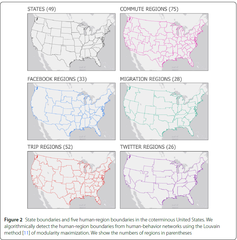
Figure 2 visualizes the regional boundaries that divide the mainland United States in six different ways. In addition to the existing state boundaries, functional regions were generated using the Louvain algorithm based on networks derived from commuting, migration, travel, Twitter, and Facebook data. The commuting network resulted in the most granular division with 75 regions, while the Twitter and migration networks produced broader partitions with 26 and 28 regions.

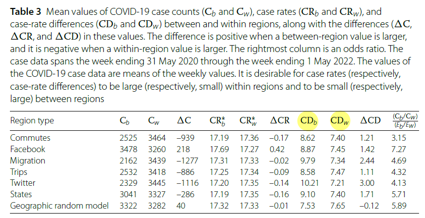
According to Table 3, the commuting-based regions exhibited the highest number of within-region infections (Cw) and the largest differences in infection rates between regions (CDb), effectively capturing a structure in which disease transmission remained confined within boundaries. In contrast, although the migration-based regions had the highest CDb values due to clear separations between regions, the internal coherence was weaker, as reflected in the relatively small within-region infection rate differences (CDw). The Facebook-based regions showed minimal differences in infection rates both within and between regions and had lower Cw values, indicating limited effectiveness as functional boundaries.

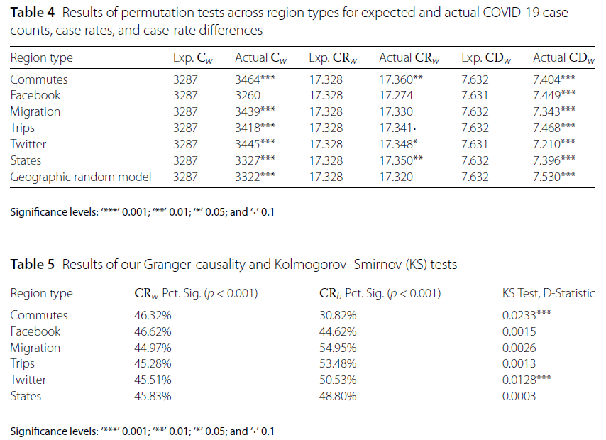
This pattern was also supported by the permutation test results in Table 4. For the commuting, migration, and trip-based regions, the actual Cw values were significantly higher than the expected values under random assignment (p < 0.001), while CDw values were consistently lower—suggesting that these regions formed tightly connected internal structures. In contrast, Facebook-based and random regions showed few statistically significant differences, confirming that they did not function as effective transmission boundaries.

Table 5 further evaluated temporal transmission dynamics using Granger causality and the Kolmogorov–Smirnov (KS) test. In the commuting regions, Granger causality was high within regions (CRw) but low between regions (CRb), indicating that infections tended to propagate internally rather than across boundaries. Twitter regions demonstrated a similar temporal trend but with weaker spatial separation. The KS test also showed the largest D-statistic values for commuting and Twitter-based regions, highlighting a clear difference in infection rate distributions inside versus across regional boundaries.

Taken together, the analysis shows that commuting-based regions performed best as functional units for delineating the spread of infectious diseases. Trip- and state-based regions also showed moderate boundary effectiveness, while Facebook-based and random regions were ineffective in structurally separating transmission patterns.

Community Detection California

📦 Data Introduction

Data Sources

1. County shapefile
COUNTY_2019_US_SL050_Coast_Clipped.shp
Used for visualizing county-level community partitions on a choropleth map

2. MSA shapefile (Metropolitan Statistical Areas)
CBSA_MSA_2019_US_SL310_Coast_Clipped.shp
Used to compare community-detected regions with official administrative boundaries

3. Socioeconomic data
R13859119_SL050.csv with data dictionary R13859119.txt
Includes variables such as population, income, education, unemployment, and more
Aggregated by community cluster to analyze group differences

4. Migration flow data
county-to-county-2016-2020-ins-outs-nets.xlsx
Includes in-migration, out-migration, net, and gross flow between counties

Data Pre-processing

1. Link

Read Excel file from the “California” sheet and keep only the first 9 columns.

link = pd.read_excel('county-to-county-2016-2020-ins-outs-nets-gross.xlsx', sheet_name='California', skiprows=2)

link = link.iloc[:, 0:9]

link.columns = [
    'state_code_a',
    'county_code_a',
    'state_code_b',
    'county_code_b',
    'state_name_a',
    'county_name_a',
    'state_name_b',
    'county_name_b',
    'weight'
]

Filter out flows with weight less than or equal to 50 to reduce noise

link = link[(link['state_name_a'] == 'California') & (link['state_name_b'] == 'California') & (link['weight'] > 50)]

2. Node

Filter for California counties only (Geo_STATE == 6)

node = node[node['Geo_STATE'] == 6]

Select only the columns required to compare community-level differences in population, race, education, income, and commuting patterns.

node = node[[
    'Geo_FIPS',
    'Geo_QName', 
    'Geo_STATE',
    'Geo_COUNTY',
    'SE_A00001_001',  # Total population
    'SE_A03001_002',  # White Alone
    'SE_A03001_003',  # Black or African American Alone
    'SE_A03001_005',  # Asian Alone
    'SE_A00002_002',  # Population density
    'SE_A12001_005',  # Bachelor's degree
    'SE_A17005_003',  # Unemployed
    'SE_A14006_001',  # Median household income
    'SE_A09003_001'   # Average commute time
]]

🧭 California County-to-County Migration Network

The network displays the strongest migration links among California’s 58 counties, rather than the full set of connections.

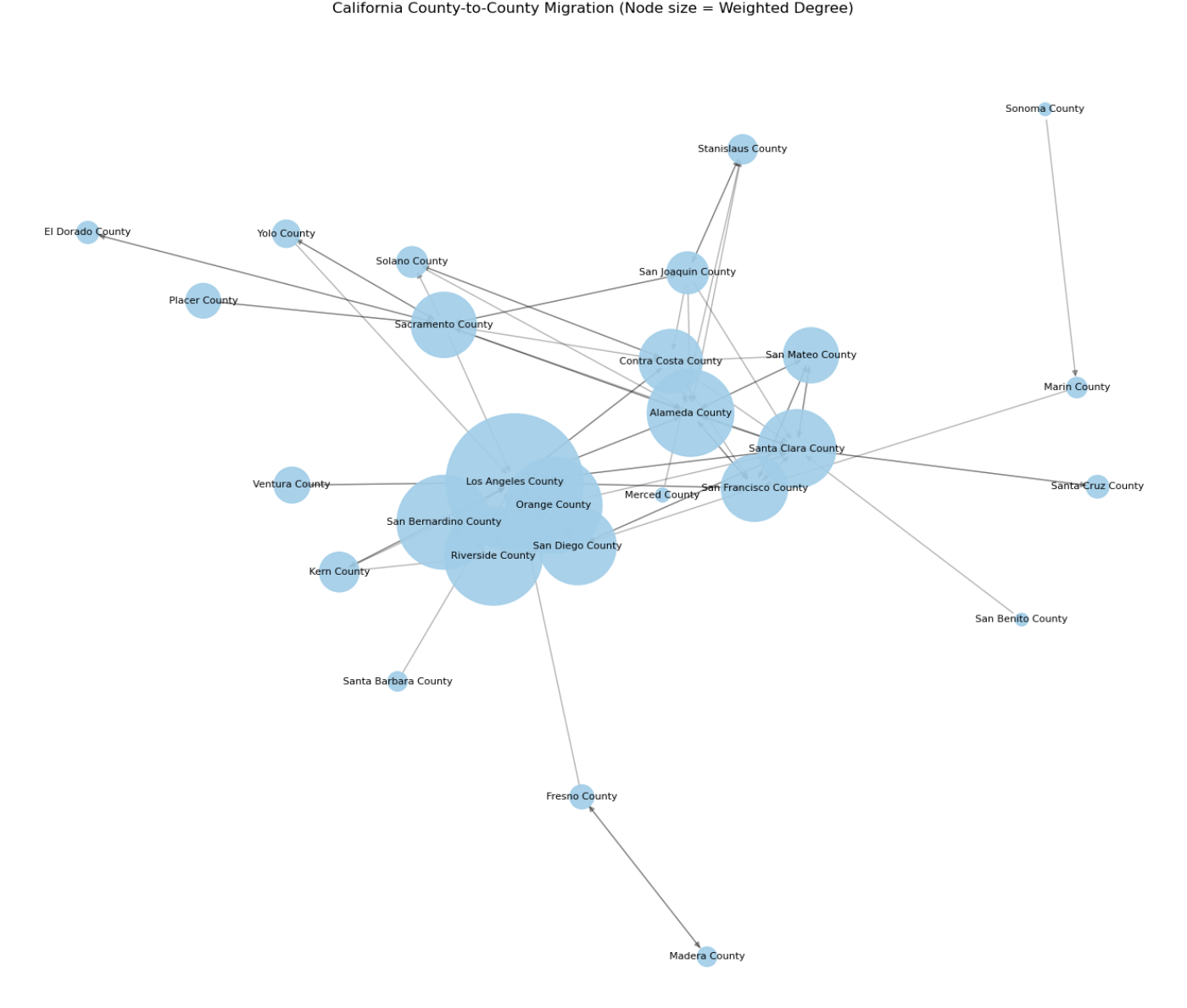
Los Angeles County appears as the largest node by far, indicating that it serves as the most active migration hub within California
→ It plays a central role with high volumes of both in-migration and out-migration

Riverside, Orange, San Diego, and San Bernardino Counties, all located in Southern California, are densely connected around Los Angeles
→ This reflects strong migration flows within the greater metropolitan area

💡 Algorithms

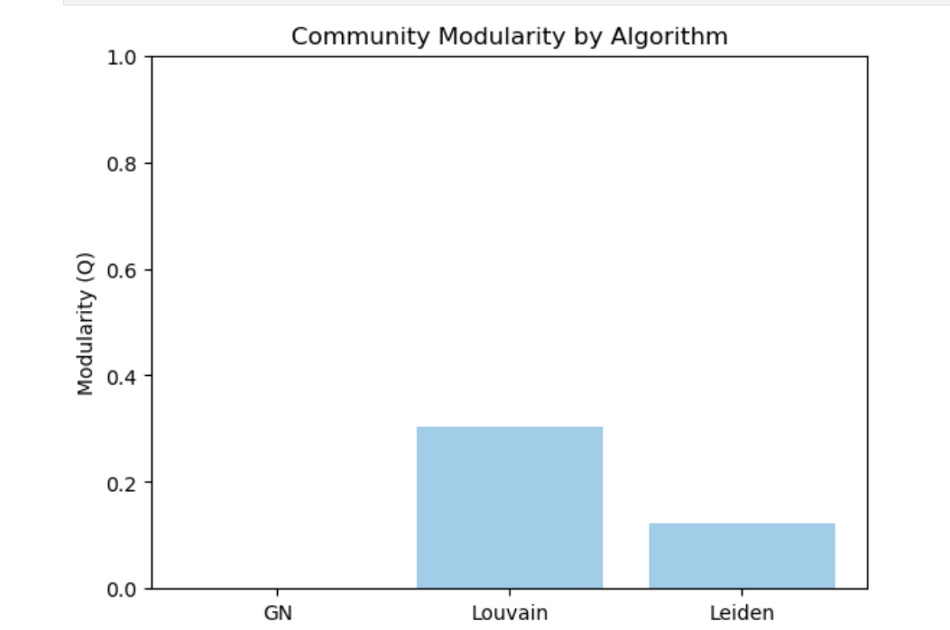
By comparing several community detection algorithms, the most effective way to divide regions within California was evaluated. The algorithms used in the comparison include Girvan–Newman (GN), Louvain, and Leiden. Each algorithm explores the network structure differently, and their performance was compared based on Modularity (Q).

The graph above shows the modularity (Q) values calculated after applying each algorithm. Modularity quantifies how well a network distinguishes between internal and external regional structures—higher values indicate clearer community boundaries.

1. Girvan–Newman: Produced the lowest modularity. Although it generates many divisions due to its tree-based structure, the regional separation is weak.

2. Leiden: A faster and more efficient algorithm than Louvain, but in this dataset, it resulted in relatively low modularity.

3. Louvain: Achieved the highest modularity (Q ≈ 0.3), effectively capturing strong internal connectivity and weak external links.

Based on these results, the Louvain algorithm was selected for dividing communities in California. The following map illustrates the regional boundaries derived from this approach.

🧠 Visualization

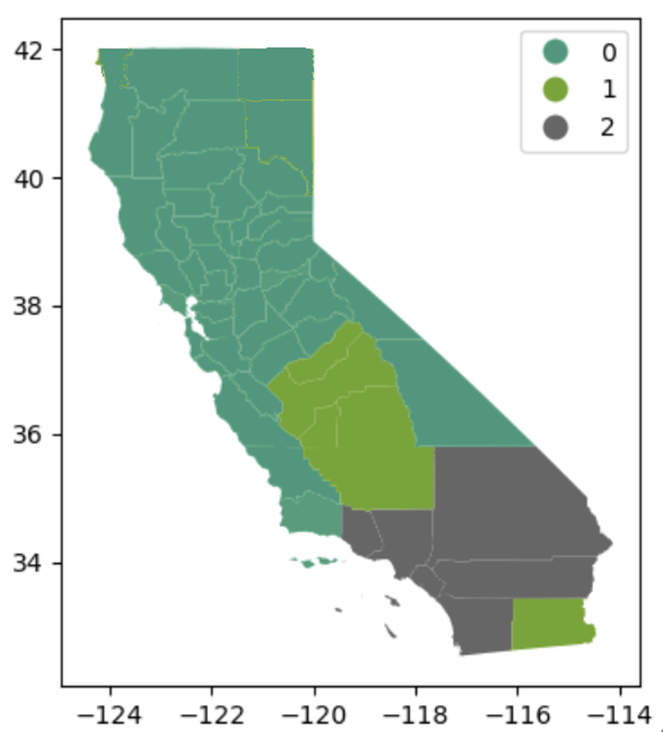
Louvain Map

This map clearly separates Southern, Central, and Northern California, and each community has a geographically continuous and interpretable boundary structure. It is highly likely to be utilized as a policy unit, especially with clear divisions centered around metropolitan areas (e.g., LA, Bay Area).The Louvain algorithm works in a way that maximizes Modularity, in which case the highest modularity value was recorded (Q ≈ 0.3). This map clearly separates Southern, Central, and Northern California, and each community has a geographically continuous and interpretable boundary structure. It is highly likely to be utilized as a policy unit, especially with clear divisions centered around metropolitan areas.

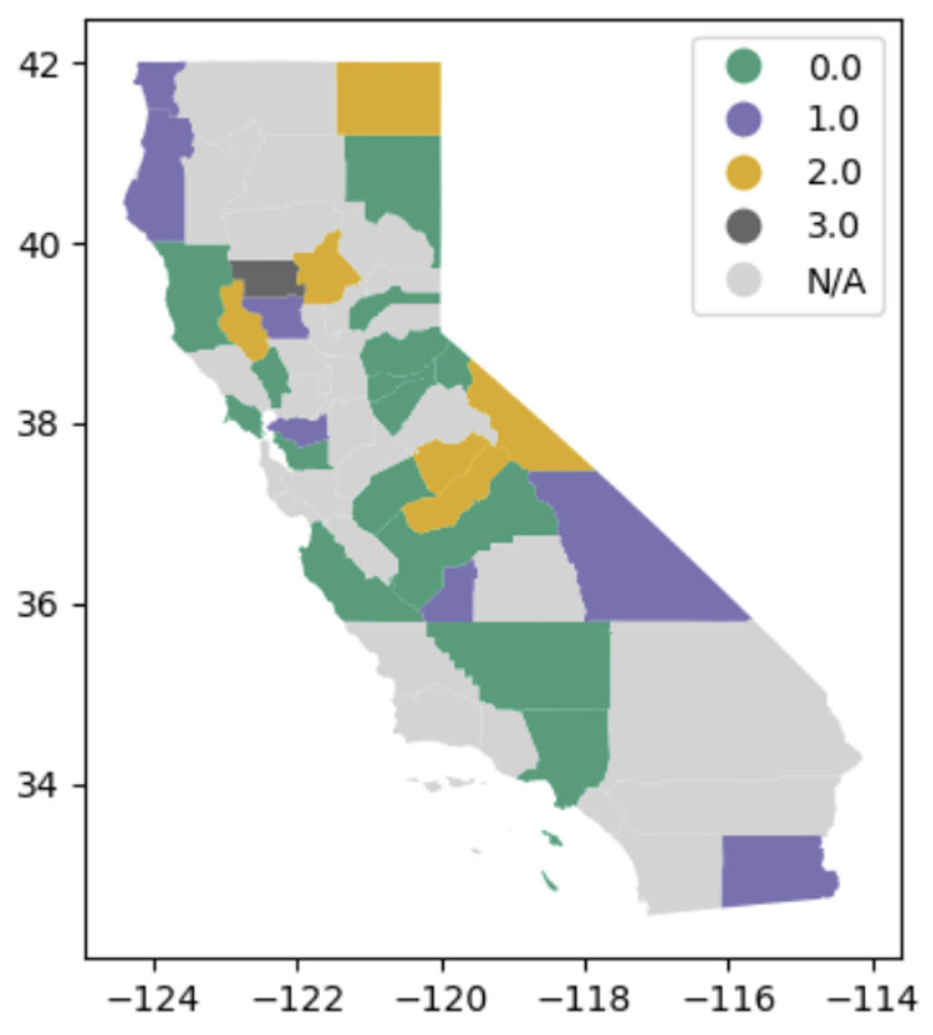
Leiden Map

The Leiden algorithm formed relatively more granular compartments. However, some communities are located in geographically dispersed locations and lack spatial continuity. It is difficult to interpret as a real policy unit because there are many cases where counties of the same color are far from each other. Furthermore, counties marked with grey (N/A) on the map are not part of any community, suggesting that the algorithm is not fully aware of their connectivity. Given that these unclassified regions are included, the Leiden algorithm may exclude some counties or cause incomplete community configurations

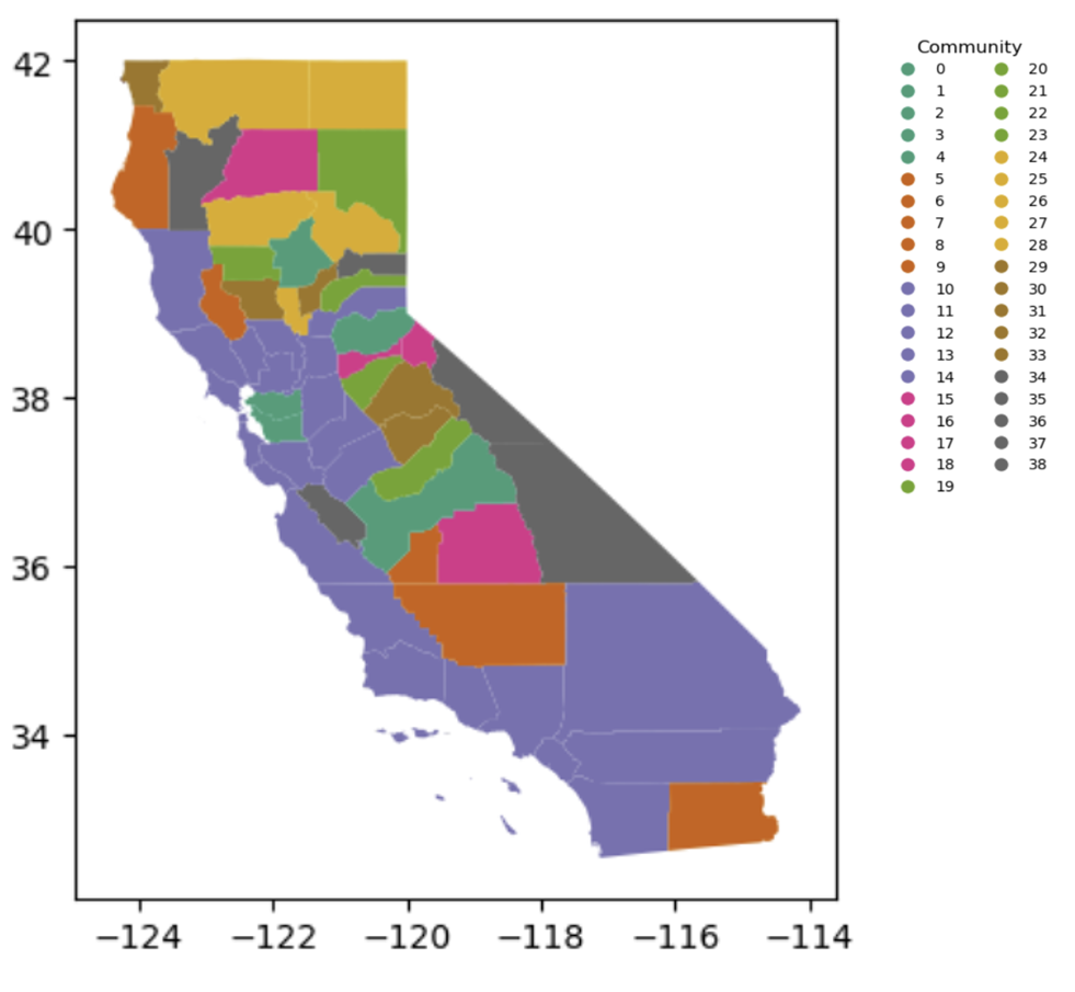
Girvan–Newman Map

Since the algorithm divides the network based on edge betweenness, it works by iterating the segmentation while removing central nodes with many connections. The result is over-divided into a total of 39 communities, which shows that the algorithm tends to over-divide complex structures. Some communities are composed of several counties that are separated from each other, resulting in a significant drop in geographic continuity. This means that the internal connectivity is not strong and the distinction between communities is unclear, indicating that it does not reflect the practical community structure well. Therefore, Girvan-Newman reveals the limitations that it is not suitable for complex real-world network structures.

Choropleth Maps

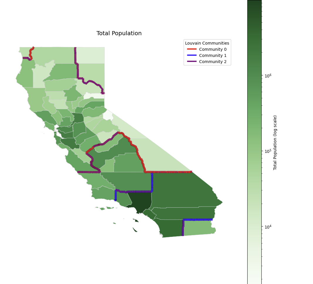
Total Population

This is a logarithmic scale map of the total population by county. The darker the green, the greater the population, and the greater the concentration of the population in Southern California (e.g., LA, San Diego) and the Bay Area. The Louvain community boundaries (Red, Blue, and Violet) somewhat correspond to the distribution of the population, but they do not match perfectly, raising the need for a regional reset.

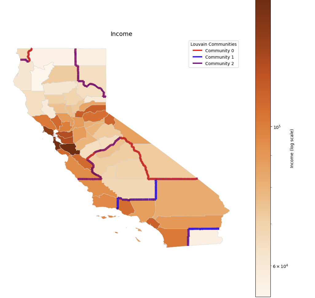
Income

A map of median income by county. High-income areas are marked in dark brown, and high-income areas concentrated around the San Francisco Bay Area are prominent. While the Louvain community boundary has well grouped some high-income areas into one community, there are cases where some low-income and high-income areas are included in the same community, indicating that there is a limit to setting boundaries that reflect income differences.

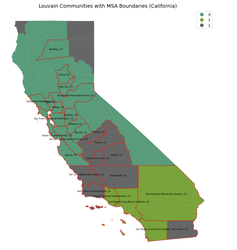
Louvain Communities with MSA Boundaries (California)

Community 0: A community centered around Northern and coastal areas of California, including the San Francisco Bay Area, Sacramento, Santa Rosa, and more. With strong connectivity between metropolitan cities and a relatively uniform network structure in the surrounding areas, functional cohesion is high.

Community 1: The region centered around Southeastern California, including Riverside, San Bernardino, and San Diego. While the big cities are adjacent, they have high internal connectivity, acting as a single unified regional unit. They are characterized by high population density and active mobility.

Community 2: The interior central region of California covers major cities such as Fresno, Bakersfield, and Visalia, but also covers some of the northern low-density areas. Though geographically dispersed, it forms an independent network internally, so it focuses on intra-regional connections rather than inter-regional interactions.

🔍 Explore Communities by Race (Boxplot)

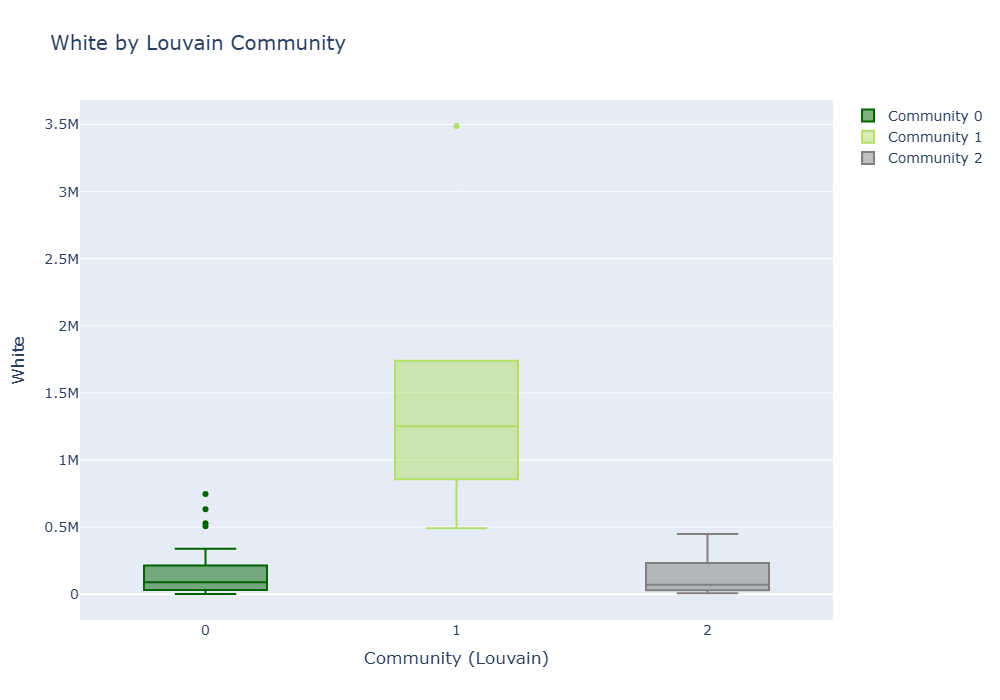
White

Community 1 has a significantly higher white population than other communities. In particular, one county includes outliers with a white population of more than 3.5 million. On the other hand, Community 0 and 2 show lower overall values, and the population distribution is also relatively narrow. This suggests that Community 1 includes counties with large populations and a high percentage of white people.

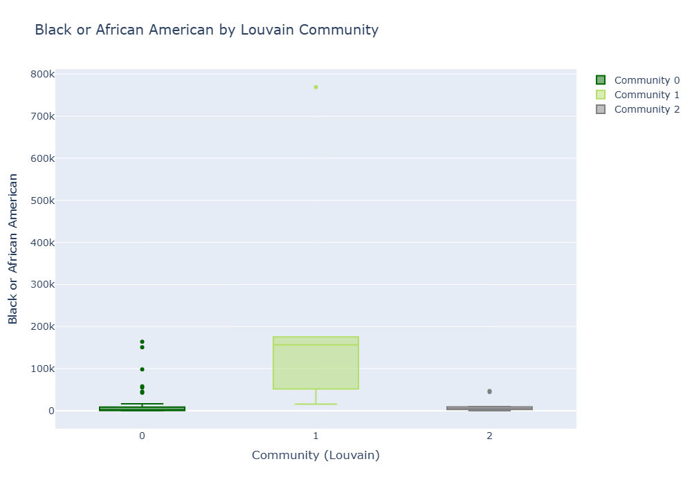
Black

The black population is also highest in Community 1, but it is not as extreme a difference as the white population. Community 0 has many outliers, and it shows various values. Community 2 has an overall consistent distribution at a low level. This means that the black population is concentrated in some of the major counties in Community 1.

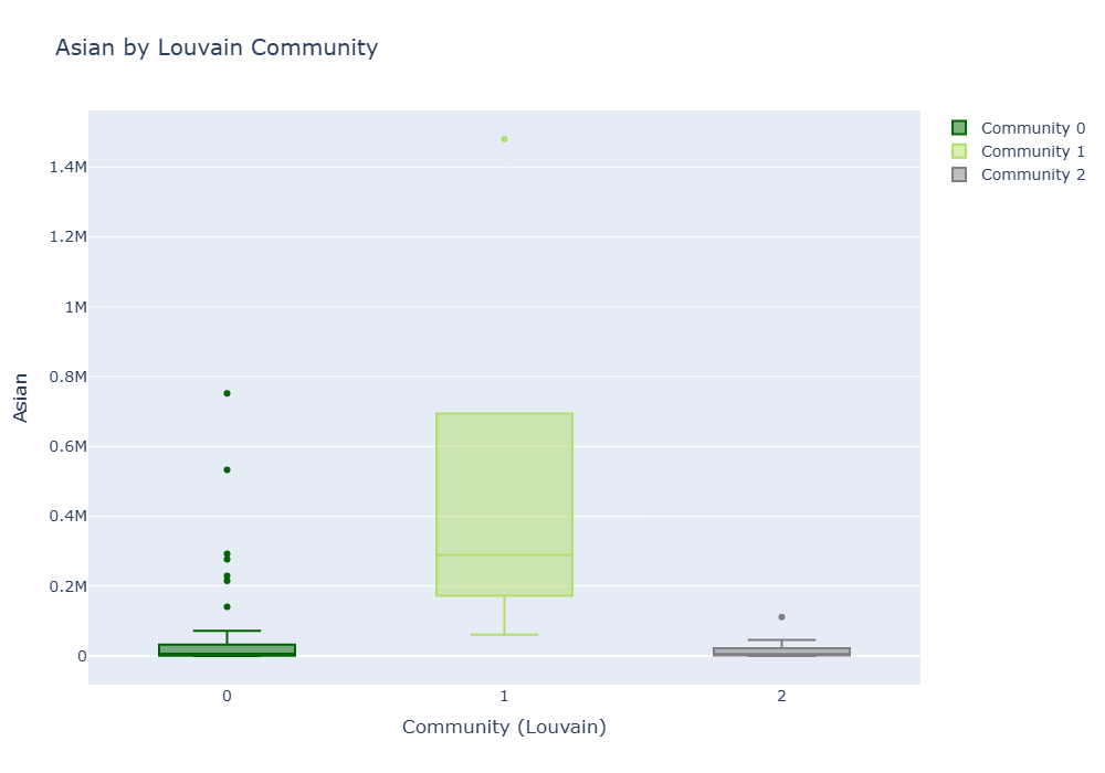
Asian

In terms of Asian population distribution, Community 1 also has the highest distribution range and there are many high outliers. This seems to be because it includes metropolitan areas such as Bay Area and Los Angeles. Communities 0 and 2 show a relatively low and uniform distribution, which can be interpreted as an area with a small or evenly distributed Asian population.

Comparison of race distribution among communities (comprehensive interpretation)

Community 1 has the highest racial population size overall. It has the largest median and distribution range among all three races (white, black, and Asian), and it also includes millions of outliers, especially for whites and Asians. This is consistent with the fact that Community 1 includes large urban areas and densely populated areas (e.g., LA, Bay Area).

Community 0 tends to be relatively evenly distributed among different races. Outliers exist in some cases, but overall variance is not large, and there is a low median for all three races. This is likely a structure that includes a large number of medium-sized cities or suburbs.

Community 2 shows the lowest ranges and medians for all three races. Counties with smaller populations themselves are clustered, and the distribution by race is also limited. This means that they contain relatively geographically isolated or sparsely populated areas.

📊 Statistical Analysis (Mann-Whitney U & Kolmogorov-Smirnov)

The Mann-Whitney U test and Kolmogorov-Smirnov (KS) test were used together in this analysis to more precisely compare the difference in population composition between communities divided by the Louvain algorithm. The Mann-Whitney U test is a nonparametric test that checks whether the difference in median value between two groups is statistically significant, and is useful even when the population is small or the distribution is skewed because it is calculated on a ranking basis without assuming a normal distribution. On the other hand, the KS test evaluates the similarity of the overall distribution form by using the maximum difference between the cumulative distribution functions of the two distributions, and is effective when the mean or median values are similar, but there may be differences in distribution width or tail. Therefore, by using the two tests together, not only the simple difference in location but also the structural difference in the overall distribution can be identified, so that the statistical difference in race composition between communities can be evaluated more reliably.

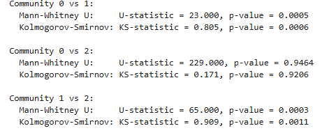
White

Community 0 vs 1
There is a significant difference between the two groups (p<0.001). The KS-statistic value (0.805) indicates that the form of the distribution is very different.

Community 0 vs 2
No statistically significant difference (p ≈ 0.94). White population distribution between the two communities is similar.

Community 1 vs 2
A distinct difference exists (p < 0.001). KS-statistic is also a very large value of 0.909.

-> Community 1 has a very large white population compared to other communities. Community 0 and 2 are relatively similar.

Black

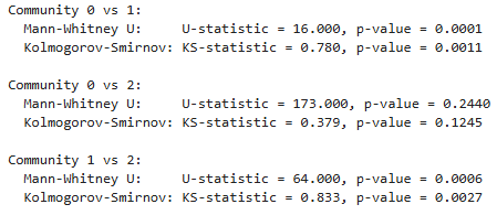
Community 0 vs 1
Significant differences exist (p < 0.001). The two groups are markedly different in the Black population distribution.

Community 0 vs 2
No significant difference (p ≈ 0.24). Black population distribution similar.

Community 1 vs 2
Significant difference (p < 0.001). KS-statistic is also very large, 0.833.

-> Community 1 also has a larger Black population than other groups. Community 0 and 2 are similar in distribution.

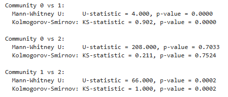
Asian

Community 0 vs 1
The distribution is very different, and the difference is also significant (p < 0.001). KS-statistic 0.902.

Community 0 vs 2
No significant difference (p ≈ 0.70). Distribution is also similar.

Community 1 vs 2
A very significant difference (p < 0.001), a completely different distribution with KS-statistic = 1.000.

-> The Asian population also has a markedly large number of Community 1. Community 0 and 2 have little difference in terms of the Asian population.

Comprehensive conclusion

Community 1 shows distinct differences from other groups in all of the White, Black, and Asian populations, and can be seen as the largest and most diverse region. Community 0 and 2 have a similar distribution for each race, and are generally interpreted as small and highly homogeneous areas. In many cases, KS statistics are high, so it can be important to consider that the difference in distribution shape itself is large in addition to the simple average.

🧾 Summary and Key Insights

Through this study, it was confirmed that functional communities based on county-to-county movement patterns in California reflect more distinct socioeconomic characteristics and structures than traditional administrative boundaries. In particular, Community 1, identified by the Louvain algorithm, stood out from other regions in terms of racial diversity and population size due to the dense demographic structure and unique social dynamics of Southern metropolitan areas, including Los Angeles and San Diego. In contrast, Communities 0 and 2 tended to have smaller populations, more uniform racial compositions, and included more isolated or low-density areas. The analysis of socioeconomic indicators revealed that Community 0 had the highest levels of income and education, largely attributable to the inclusion of the San Francisco Bay Area and other affluent northern regions. Community 2 consisted mainly of rural or mid-sized counties, characterized by lower income, lower education levels, and sparse populations. These patterns suggest that functional boundaries based on real human movement and interaction may provide a more meaningful regional classification than simple geographic proximity. These findings suggest that movement-based communities can serve as more practical units for policy-making, urban planning, and the allocation of social services than conventional administrative divisions. For instance, efforts to prevent disease transmission or reduce regional inequality could be more accurately targeted when using these functional community boundaries. Future research could expand on this approach by incorporating longitudinal analysis of how communities evolve over time and integrating additional socioeconomic variables. This would further enhance the explanatory power and practical value of community-based spatial analysis.